AC Simulation
Using the Analog Design Environment (ADE)
- In the toolbar, select Tools → Analog Environment.
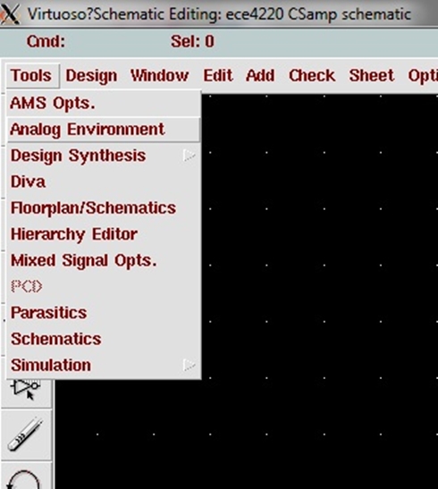
Figure 1. Open ADE
- If you need to use the models from the functional library (which we won't use in this tutorial) you have to add the model library. Let's go ahead and add it for educational purposes. In the ADE, go to Setup → Model Libraries. Add the following file (to paste in Cadence, middle click on the mouse - i.e. press down on the mouse's scroll wheel). Don't forget to press OK once it's added.
Model Library File: $CDS_HOME/tools/dfII/etc/cdslib/artist/functional/allFunc.scs
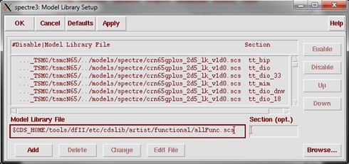
Figure 2. Add the model library
- Immediately save this state so that you don't have to add the library file every time: Go to Session → Save State... Now save it under "Cellview" (so that it will be accessible from the library manager). Leave the name as "spectre_state1" and press OK. (Next time you use the ADE for a different cellview, load a previous state from another cell to copy the library files. Then, save the new state to the current cellview and begin setting up the design environment.)
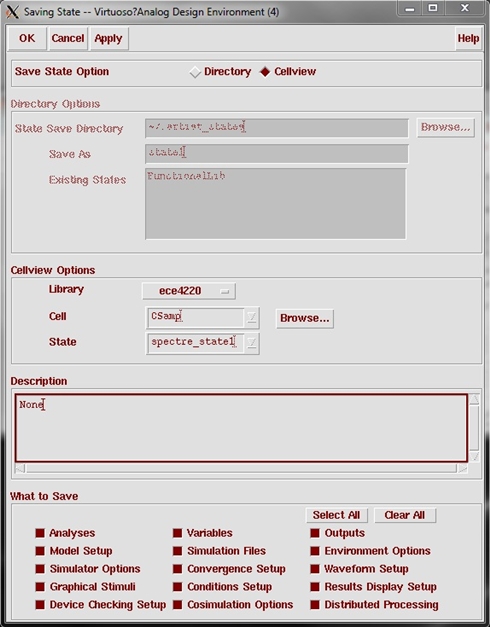
Figure 3. Save the state in your cellview
- Now let's update the "Design Variables" that we used for several parameters. In the ADE, select either the "Edit Variables" icon on the right or Variables → Edit from the toolbar.
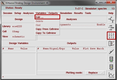
Figure 4. Edit variables
- In the next window, select "Copy From" next to "Cellview Variables" on the bottom. The variables we entered should populate the table to the right. Select each variable and "Change" the value to those shown in the figure below. select OK when completed.
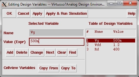
Figure 5. Update variable values
- Next, the analysis is chosen. Select "Analysis->Choose", and select "dc". Enable "Save DC Operating Point" and press Apply. You only need to add this analysis if you plan on accessing that data after simulation. Note that an analysis can be enabled or disabled by toggling the "Enabled" button at the bottom of the analysis setup.
- Now select "ac" and sweep frequency from "1" to "1G". Press OK.
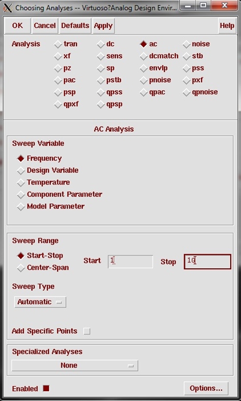
Figure 6. Setup an ac sweep
Using the Calculator to Setup Outputs
- The last thing to do is to setup our outputs. Select "Outputs->Setup", and next to "Calculator" press "Open". In the calculator, select Options and uncheck "Set RPN".
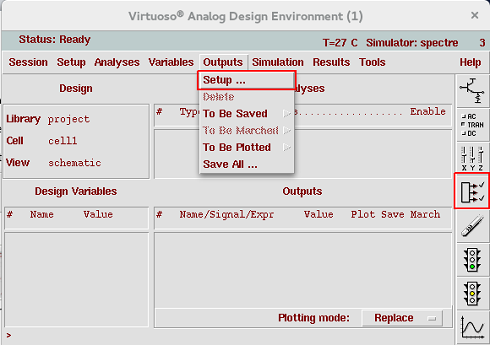
Figure 7. Setup
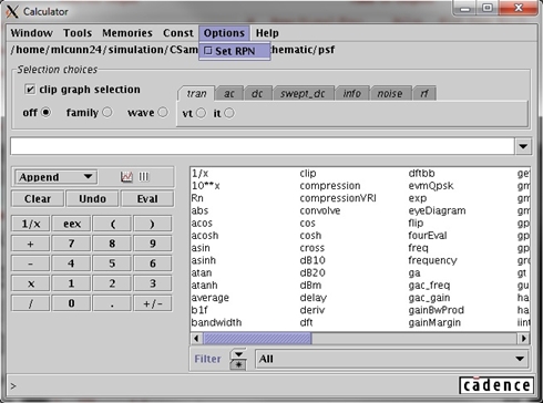
Figure 8. Calculator
- Now go to the "ac" tab and select "vf" (this is a voltage quantity vs. frequency). Place your cursor in the box and type "dB20(". Then, with "vf" selected, click on the output net (Vo) in your schematic. Add a forward slash to divide and then select the input net (Vi). Add a closing parenthesis as shown below.
NOTE: Remember to press "Esc" next time you enter the schematic (after finishing with the calculator) to cancel the calculator selection function.
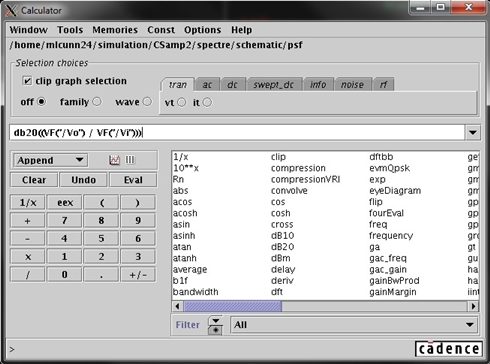
Figure 9. Setup an equation
- Without closing the calculator, go back to the outputs setup window and press "Get Expression". In the name box type "Av" then select Add and OK.
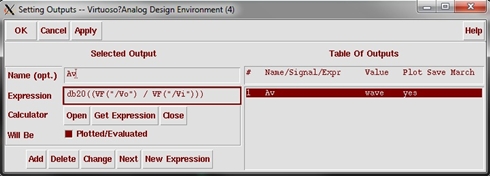
Figure 10. Output setup
- Save this session for future use. Session → Save State..., make sure cellview is selected and the correct library, cell and state name are selected, then press OK. Select OK if prompted to overwrite.
NOTE: When saving a state, make sure all plots are closed or they will be saved as part of the state (and are reopened when loading that state).
Running the Simulation
- To run the simulation, press the green traffic light icon (Netlist and Run) located near the bottom right corner. Make sure that you have checked and saved (Shift + x) your schematic or simulation will not run. When the simulation is successfully running an output log file will popup. Once completed, the output(s) will be plotted.
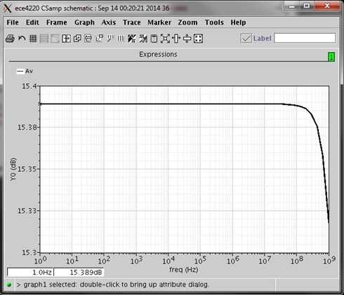
Figure 11. Simulation plot
NOTE: You can change the color, thickness, and other trace attributes by double clicking on the legend icon. Also, you can add a marker by pressing "m" and then add a delta marker (relative to the first marker point) by pressing "a".
Additional Comments
In the ADE, some other helpful options are available.
- Select Results → Annotate → DC Node Voltages. This displays net voltages on the schematic.
- Results → Direct Plot → Main Form... allows for outputs to be plotted after simulation. If you enable "Add To Outputs" then the output will be added to the ADE outputs so that it can be plotted automatically. Note that currents are usually not saved. This can be fixed in Outputs → Save All... by selecting "all" next to "Select device currents" and setting the subcircuit level to something like 7. Otherwise, the next way is to save the output via an equation.
- Results → Print → DC Operating Points will display information about the device that is selected. If the MOSFET is selected, important values such as gm, capacitances, currents, power dissipation, etc. are displayed.

MICS IAP Members